Tutorial - Backtesting
If you are completely new to TFire it is recommended to look at Tutorial - Basic Analysis of Time Series Data first.
Setting up Scoring
The decision of when to buy or sell an asset is done by Scoring the asset. To construct a Scoring we start with a slightly altered version of the setup from Tutorial - Basic Analysis of Time Series Data.
TFire> tickers = ["MMM", "AOS", "ABT", "ACN", "ATVI"];

TFire> spec = Specification(tickers, Date(2001,6,2),Date(2018,6,8); extend_back=600);

TFire> collection = setup_collection(spec);
Let's now cheat and filter out all all dates that have a return after 10 days larger than the average return after 10 days. First we find out what the average return is after 10 trading days
TFire> ret = compound_return(collection, 10;flat=true);

TFire> mean_return = mean(ret)
1.0078063862992992
Here, we use the compound_return function to calculate the return after 10 days. flat=true is used to flatten the returned values into a vector. Finally, we use the mean function to get the average return after 10 days.
Now we can filter out the dates that have a return larger than the average return after 10 days. First let's create a function that returns true if a value is larger than the average return after 10 days.
TFire> function higher_than_average(args)
       x = args[1]
       return x > 1.0078063862992992
       end
then filter a copy of the original collection
TFire> cret = compound_return(collection, 10);

TFire> collection_higher = filter_collection(collection, [cret], higher_than_average;action=:keep)
We can compare the number of samples in the original collection and the filtered collectio and notice that as expected about half of the samples had a higher return than the average sample.
TFire> collection
-| Collection |- (Continuous)
Tickers: 5, MMM AOS ABT ACN ATVI
Samples: 21373

TFire> collection_higher
-| Collection |- (Continuous)
Tickers: 5, MMM AOS ABT ACN ATVI
Samples: 10759
Now it's time to create the actual Scoring.
TFire> buy_scores = BuyScores(collection_higher, 1.);This function creates a BuyScores (see Scoring) where every date contained in collection_higher, i.e. all dates that have higher than average return after 10 days, gets a score of 1.
Setting up an Initial Portfolio
TFire> from_date = DateTime(2002,1,7)

TFire> port = initialize_portfolio(collection, from_date);
Let's hold the assets for 10 days after they were bought.
TFire> position_scores = extend_scores(buy_scores, port; constant_ticks=10);This creates a PositionScores object, which has a score of 1 for every date in ScoreBuy and 10 days forward.
Propagating the Portfolio
We can propagate the initial portfolio port using the position_scores to get a PortfolioHistory.
TFire> port_prop = propagate_portfolio(port, position_scores)
-| Portfolio History |-  4135 number of steps from 2002-01-07T00:00:00 to 2018-06-08T00:00:00
Analysing the Results
To evaluate the performance of our portfolio, we begin by plotting it against a portfolio where all of the stocks available for trade are bought for equal ammount at day 1 and then held to the final day, i.e. equal weighted buy and hold. We can get this portfolio by running reference_portfolio(port_prop).
TFire> plot_portfolio(port_prop, reference_portfolio(port_prop))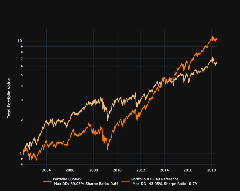 The cheating portfolio is of course significantly outperforming the buy and hold variant, with a 600x return vs 20x return over the time period.
We can add a trading fee of 1% on all trades and see what that does.
TFire> port_prop_fee = propagate_portfolio(port, position_scores; fee_type=:proportional, prop_fee=0.01)

TFire> plot_portfolio(port_prop_fee, reference_portfolio(port_prop_fee))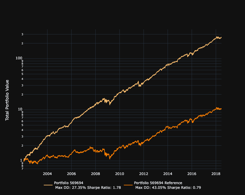
That concludes this tutorial on the basics of backtesting in TFire.